Lab sheet 6: Introduction to statistics
I have used codes from the book Dalgaard (2008) for this lab.
Descriptive statistics
x <- rnorm(50)
mean_x <- mean(x)
sd_x <- sd(x)
var_x <- var(x)
median_x <- median(x)

# Moments
library(moments)
skewness_x <- skewness(x)
kurtosis_x <- kurtosis(x)

list(mean = mean_x, sd = sd_x, var = var_x, median = median_x,
     skewness = skewness_x, kurtosis = kurtosis_x)
## $mean
## [1] 0.1626365
##
## $sd
## [1] 0.9969765
##
## $var
## [1] 0.9939621
##
## $median
## [1] 0.2662041
##
## $skewness
## [1] -0.3337814
##
## $kurtosis
## [1] 5.17371quantile_x <- quantile(x)
pvec <- seq(0, 1, 0.1)
quantile_values <- quantile(x, pvec)
list(quantiles = quantile_x, pvec = pvec, quantile_values = quantile_values)## $quantiles
## 0% 25% 50% 75% 100%
## -3.2331521 -0.3589715 0.2662041 0.6624521 2.9191401
##
## $pvec
## [1] 0.0 0.1 0.2 0.3 0.4 0.5 0.6 0.7 0.8 0.9 1.0
##
## $quantile_values
## 0% 10% 20% 30% 40% 50%
## -3.23315213 -1.07956513 -0.45383165 -0.28370927 0.04854668 0.26620409
## 60% 70% 80% 90% 100%
## 0.41526247 0.60485247 0.71271795 1.19187526 2.91914013data()
head(Nile)## [1] 1120 1160 963 1210 1160 1160summary(Nile)## Min. 1st Qu. Median Mean 3rd Qu. Max.
## 456.0 798.5 893.5 919.4 1032.5 1370.0library('ISwR')
attach(juul)
names(juul)## [1] "age" "menarche" "sex" "igf1" "tanner" "testvol"mean(igf1)## [1] NAmean(igf1,na.rm=T)## [1] 340.168summary(igf1)## Min. 1st Qu. Median Mean 3rd Qu. Max. NA's
## 25.0 202.2 313.5 340.2 462.8 915.0 321summary(juul)## age menarche sex igf1 tanner
## Min. : 0.170 No :369 M :621 Min. : 25.0 I :515
## 1st Qu.: 9.053 Yes :335 F :713 1st Qu.:202.2 II :103
## Median :12.560 NA's:635 NA's: 5 Median :313.5 III : 72
## Mean :15.095 Mean :340.2 IV : 81
## 3rd Qu.:16.855 3rd Qu.:462.8 V :328
## Max. :83.000 Max. :915.0 NA's:240
## NA's :5 NA's :321
## testvol
## Min. : 1.000
## 1st Qu.: 1.000
## Median : 3.000
## Mean : 7.896
## 3rd Qu.:15.000
## Max. :30.000
## NA's :859detach(juul)juul$sex <- factor(juul$sex,labels=c("M","F"))
juul$menarche <- factor(juul$menarche,labels=c("No","Yes"))
juul$tanner <- factor(juul$tanner,labels=c("I","II","III","IV","V"))
attach(juul)
summary(juul)## age menarche sex igf1 tanner
## Min. : 0.170 No :369 M :621 Min. : 25.0 I :515
## 1st Qu.: 9.053 Yes :335 F :713 1st Qu.:202.2 II :103
## Median :12.560 NA's:635 NA's: 5 Median :313.5 III : 72
## Mean :15.095 Mean :340.2 IV : 81
## 3rd Qu.:16.855 3rd Qu.:462.8 V :328
## Max. :83.000 Max. :915.0 NA's:240
## NA's :5 NA's :321
## testvol
## Min. : 1.000
## 1st Qu.: 1.000
## Median : 3.000
## Mean : 7.896
## 3rd Qu.:15.000
## Max. :30.000
## NA's :859juul <- transform(juul,sex=factor(sex,labels=c("M","F")),
menarche=factor(menarche,labels=c("No","Yes")),
tanner=factor(tanner,labels=c("I","II","III","IV","V")))Graphics for single data
mid.age <- c(2.5, 7.5, 13, 16.5, 17.5, 19, 22.5, 44.5, 70.5)
acc.count <- c(28, 46, 58, 20, 31, 64, 149, 316, 103)
age.acc <- rep(mid.age, acc.count)
brk <- c(0, 5, 10, 16, 17, 18, 20, 25, 60, 80)
hist(age.acc, breaks = brk)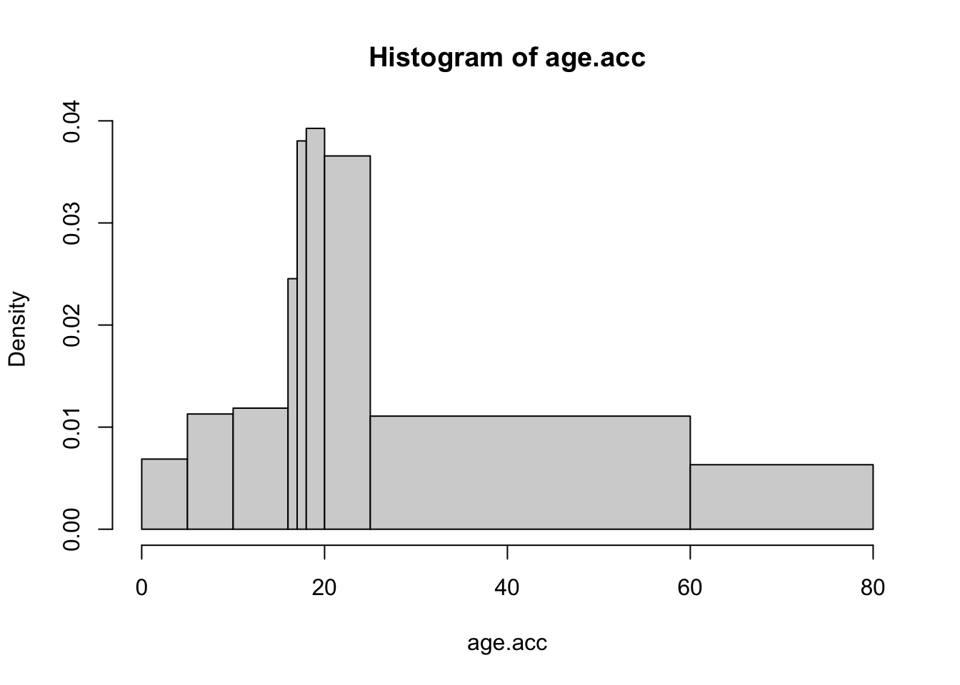
Q-Q plot
x <- rnorm(10000)
qqnorm(x)
qqline(x, col = 2,lwd=2)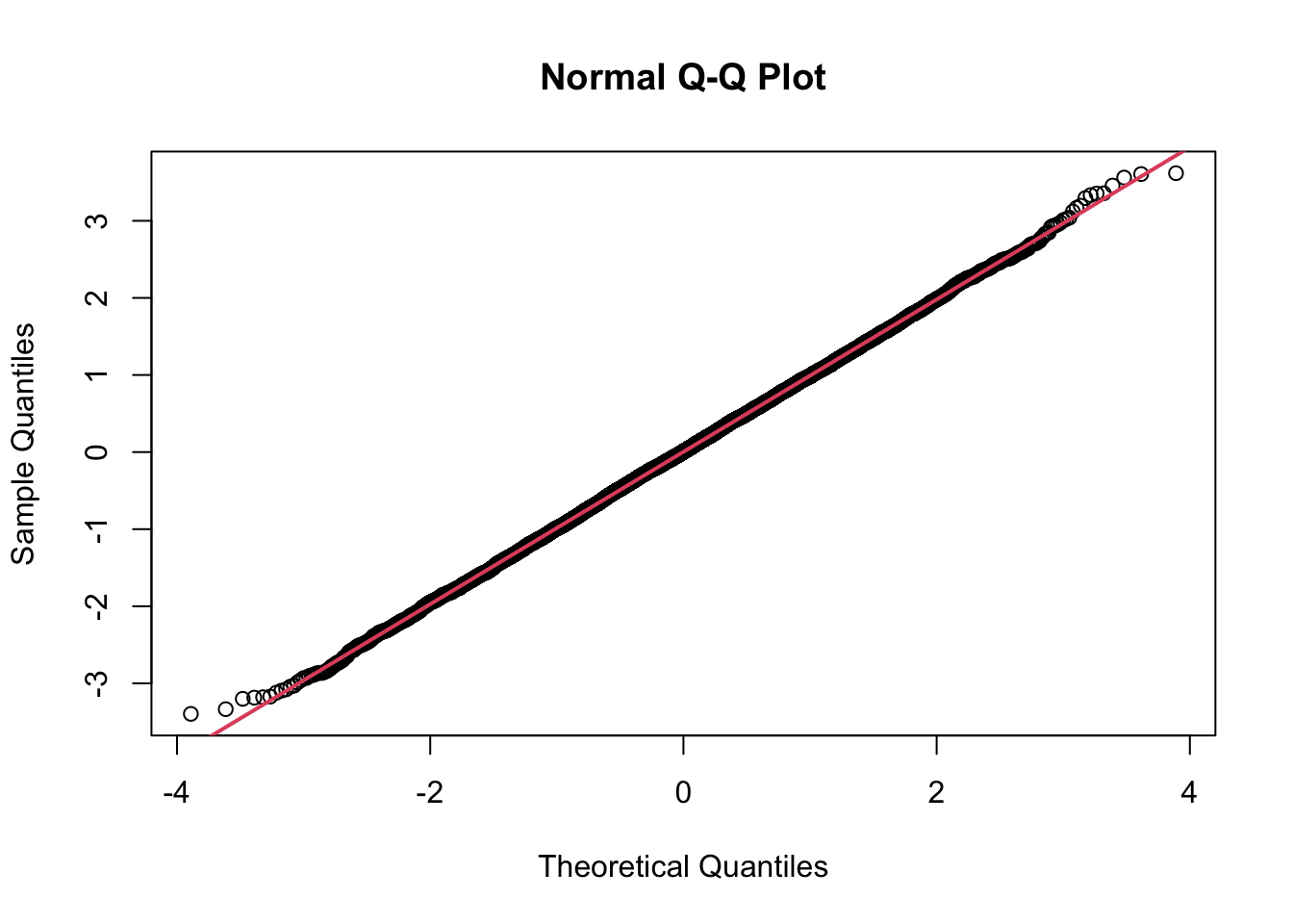
library(ggplot2)
data <- data.frame(x)
ggplot(data, aes(sample = x)) +
  stat_qq() +
  stat_qq_line(col = "red")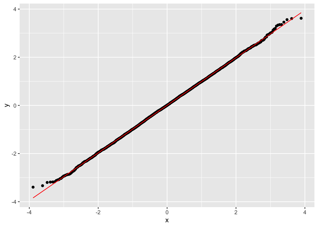
sample_data <- ToothGrowth
qqnorm(sample_data$len)
qqline(sample_data$len, col = 2, lwd = 2)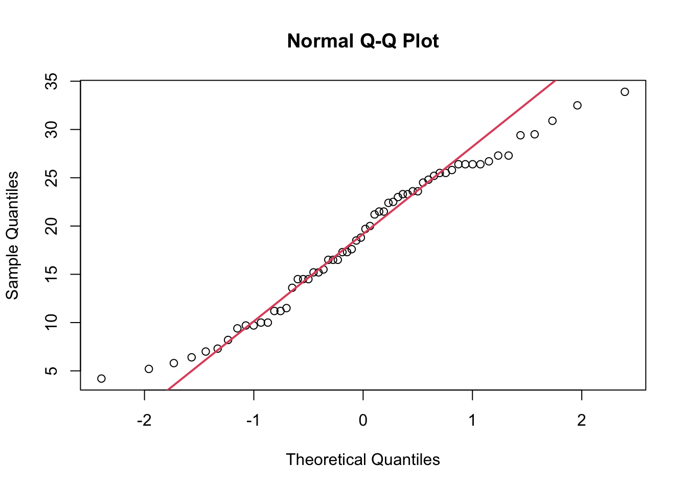
Box plot
par(mfrow=c(1,2))
boxplot(IgM)
boxplot(log(IgM))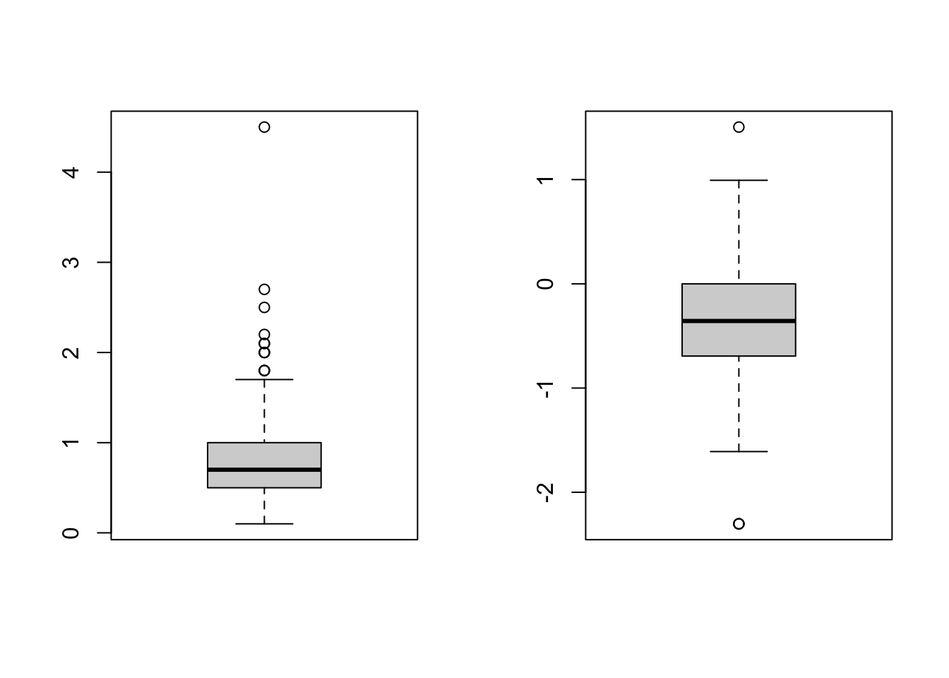
par(mfrow=c(1,1))Summary statistics by group
xbar <- tapply(igf1, tanner, mean, na.rm=T)
s <- tapply(igf1, tanner, sd, na.rm=T)
n <- tapply(igf1, tanner, length)
cbind(mean=xbar, std.dev=s, n=n)
## mean std.dev n
## I 207.4727 90.27237 515
## II 352.6714 122.59332 103
## III 483.2222 152.28664 72
## IV 513.0172 119.09594 81
## V 465.3344 134.41867 328aggregate(juul[c("age","igf1")], juul["sex"], mean, na.rm=T)by(juul, juul["sex"], summary)## sex: M
## age menarche sex igf1 tanner
## Min. : 0.17 No : 0 M:621 Min. : 29.0 I :291
## 1st Qu.: 8.85 Yes : 0 F: 0 1st Qu.:176.0 II : 55
## Median :12.38 NA's:621 Median :280.0 III : 34
## Mean :15.38 Mean :310.9 IV : 41
## 3rd Qu.:16.77 3rd Qu.:430.2 V :124
## Max. :83.00 Max. :915.0 NA's: 76
## NA's :145
## testvol
## Min. : 1.000
## 1st Qu.: 1.000
## Median : 3.000
## Mean : 7.896
## 3rd Qu.:15.000
## Max. :30.000
## NA's :141
## ------------------------------------------------------
## sex: F
## age menarche sex igf1 tanner
## Min. : 0.25 No :369 M: 0 Min. : 25.0 I :224
## 1st Qu.: 9.30 Yes :335 F:713 1st Qu.:233.0 II : 48
## Median :12.80 NA's: 9 Median :352.0 III : 38
## Mean :14.84 Mean :368.1 IV : 40
## 3rd Qu.:16.93 3rd Qu.:483.0 V :204
## Max. :75.12 Max. :914.0 NA's:159
## NA's :176
## testvol
## Min. : NA
## 1st Qu.: NA
## Median : NA
## Mean :NaN
## 3rd Qu.: NA
## Max. : NA
## NA's :713Graphics for grouped data
attach(energy)
expend.lean <- expend[stature=="lean"]
expend.obese <- expend[stature=="obese"]
par(mfrow=c(2,1))
hist(expend.lean,breaks=10,xlim=c(5,13),ylim=c(0,4),col="white")
hist(expend.obese,breaks=10,xlim=c(5,13),ylim=c(0,4),col="grey")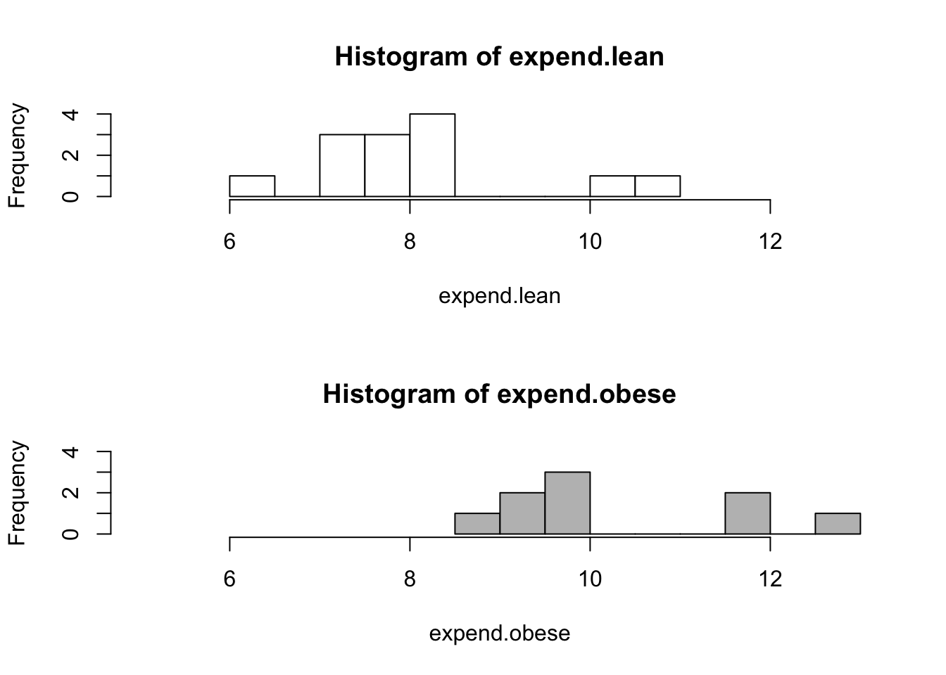
par(mfrow=c(1,1))
boxplot(expend ~ stature)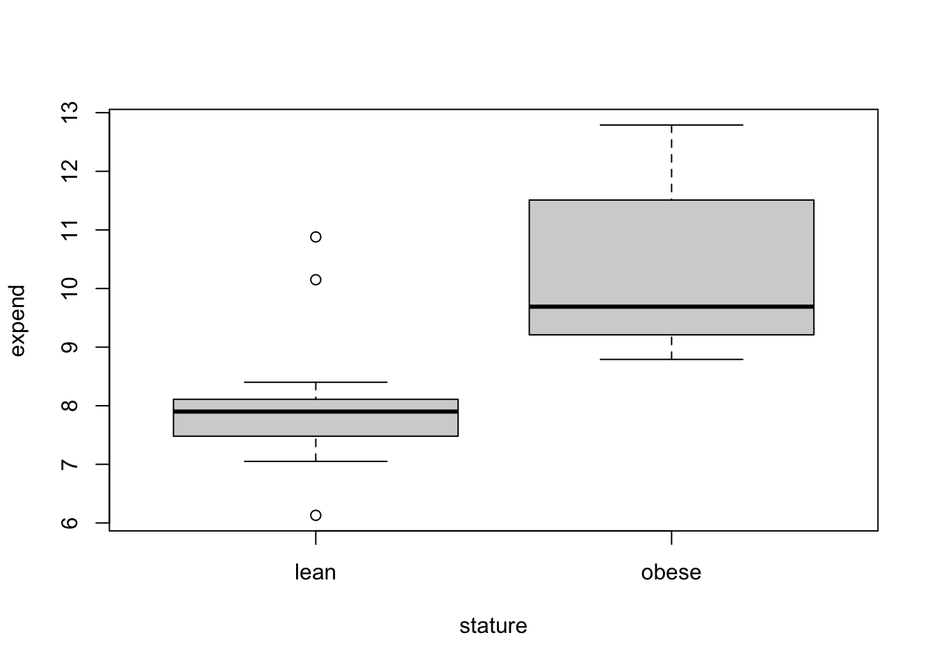 Hypothesis Testing
# One-sample t-test
t_test_result <- t.test(igf1 ~ sex, data = juul, var.equal = TRUE)
t_test_result
##
## Two Sample t-test
##
## data: igf1 by sex
## t = -5.3949, df = 1011, p-value = 8.54e-08
## alternative hypothesis: true difference in means between group M and group F is not equal to 0
## 95 percent confidence interval:
## -78.02476 -36.40325
## sample estimates:
## mean in group M mean in group F
## 310.8866 368.1006Tables
caff.marital <- matrix(c(652,1537,598,242,36,46,38,21,218,327,106,67),
                         nrow=3,byrow=T)
colnames(caff.marital) <- c("0","1-150","151-300",">300")
rownames(caff.marital) <- c("Married","Prev.married","Single")
caff.marital
## 0 1-150 151-300 >300
## Married 652 1537 598 242
## Prev.married 36 46 38 21
## Single 218 327 106 67names(dimnames(caff.marital)) <- c("marital","consumption")
caff.marital## consumption
## marital 0 1-150 151-300 >300
## Married 652 1537 598 242
## Prev.married 36 46 38 21
## Single 218 327 106 67as.data.frame(as.table(caff.marital))table(menarche,tanner)## tanner
## menarche I II III IV V
## No 221 43 32 14 2
## Yes 1 1 5 26 202xtabs(~ tanner + sex, data=juul)## sex
## tanner M F
## I 291 224
## II 55 48
## III 34 38
## IV 41 40
## V 124 204total.caff <- margin.table(caff.marital,2)
total.caff## consumption
## 0 1-150 151-300 >300
## 906 1910 742 330barplot(total.caff, col="white")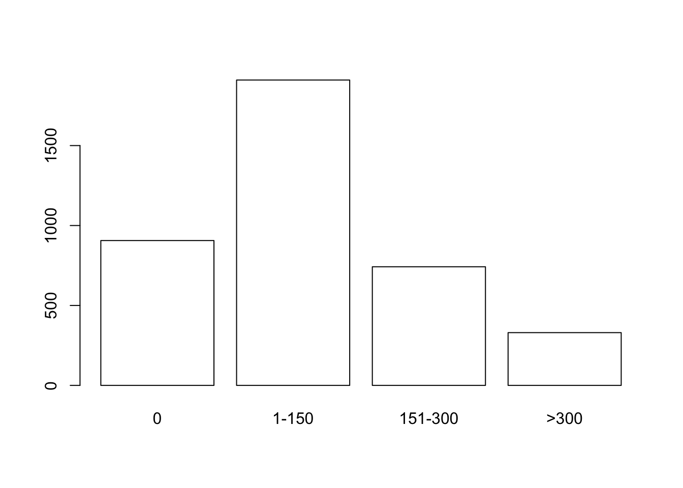
par(mfrow=c(2,2))
barplot(caff.marital, col="white")
barplot(t(caff.marital), col="white")
barplot(t(caff.marital), col="white", beside=T)
barplot(prop.table(t(caff.marital),2), col="white", beside=T)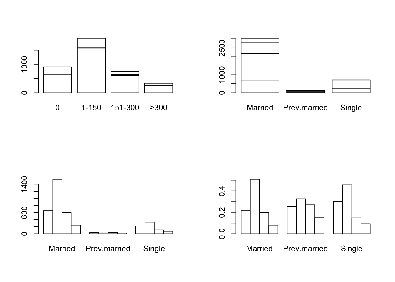
par(mfrow=c(1,1))
barplot(prop.table(t(caff.marital),2),beside=T,
        legend.text=colnames(caff.marital),
        col=c("white","grey80","grey50","black"))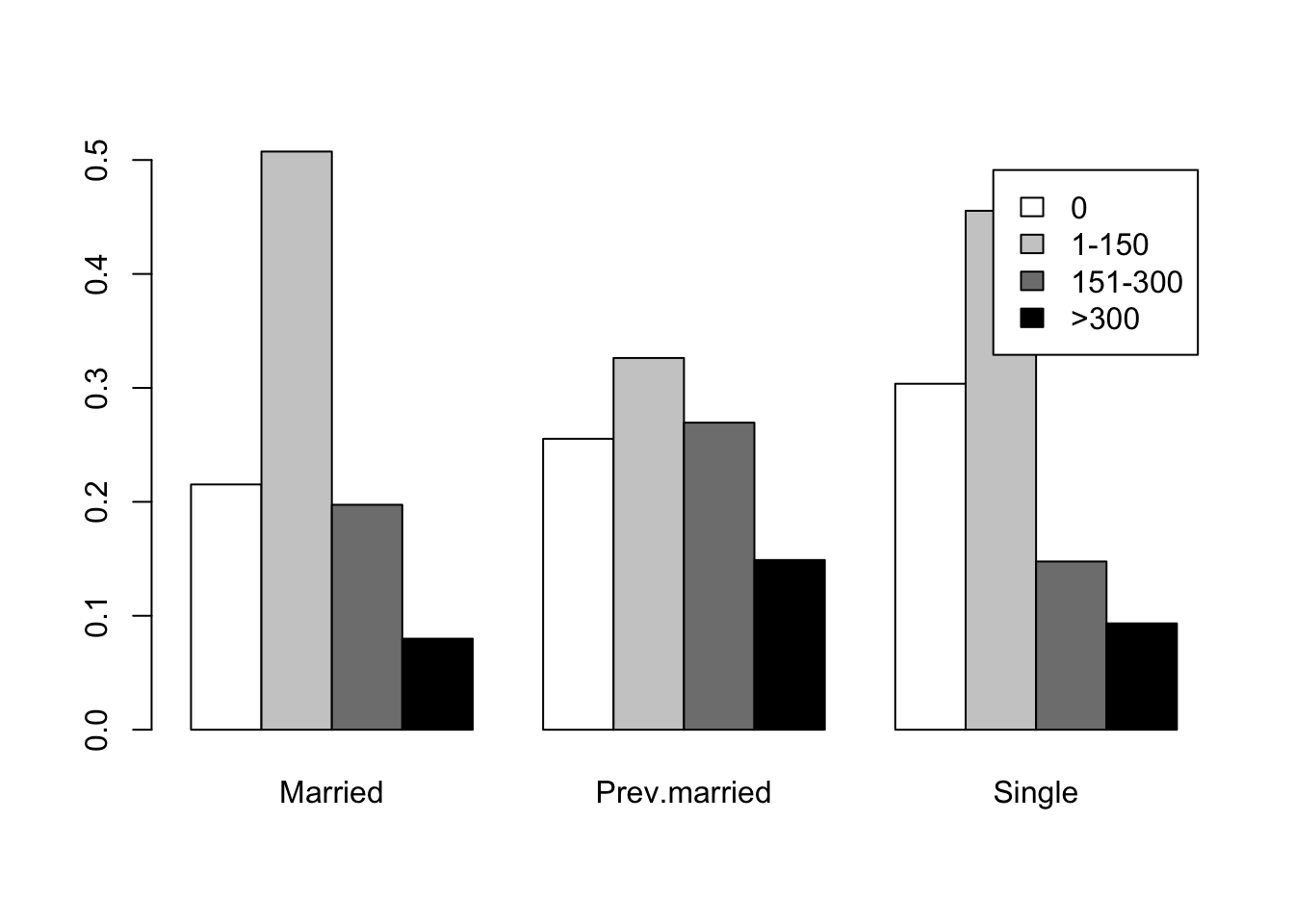
Piecharts
opar <- par(mfrow=c(2,2),mex=0.8, mar=c(1,1,2,1))
slices <- c("white","grey80","grey50","black")
pie(caff.marital["Married",], main="Married", col=slices)
pie(caff.marital["Prev.married",],
    main="Previously married", col=slices)
pie(caff.marital["Single",], main="Single", col=slices)
par(opar)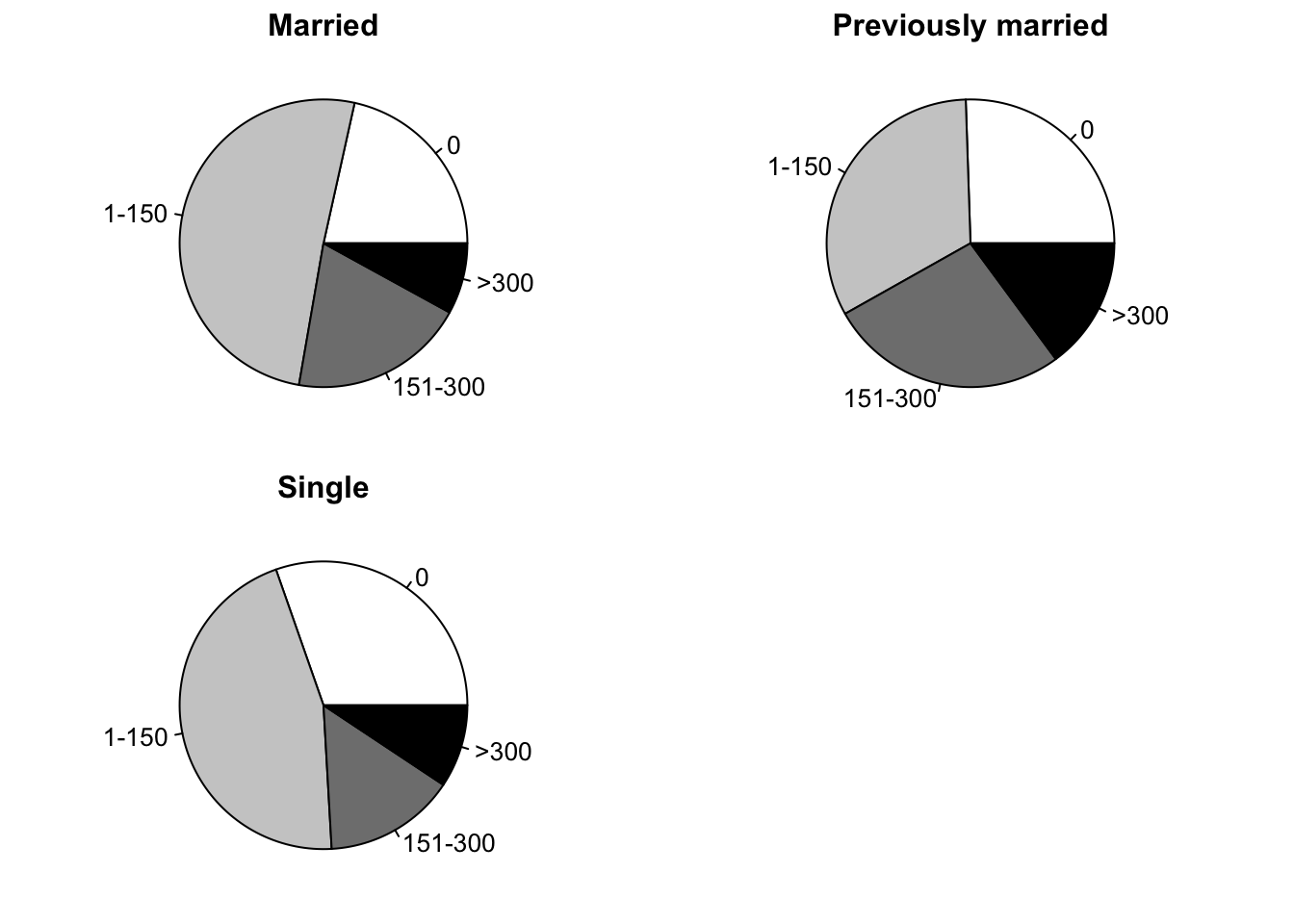
References
Dalgaard, Peter. 2008. Introductory Statistics with R. Springer New York. https://doi.org/10.1007/978-0-387-79054-1.